Earlier this year, a blog post on bitwise analysis by Jay Gattuso of NZNL reminded me that I had never got around to writing up some similar exploratory work I did while I was working on the SCAPE project. A month later, I presented a summary of the work at the SPRUCEdp Unified Characterisation Hackathon, where I attempted to explain how bitwise analysis can be used to help understand digital resources and how software tools operate upon them. This document is an attempt to outline the approach and initial results in more detail, showing how the bit-level sensitivity of various JP2 tools can be effectively mapped and compared.
Bitwise Analysis
At heart, the approach is a very simple brute-force analysis: we systematically flip each and every bit in a source bitstream and observe whether a given software process notices the change. This allows us to build up a map of how the data the the tool interact.
To look at JPEG2000 tools, we first need to create a small test image, such as this 16px square fragment of a photograph:
We then convert it to the format of interest, in this case a 773 byte JP2 file (created via a PPM derived using ImageMagick, which was then passed through Kakadu).
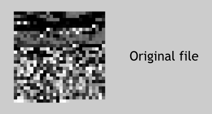
If we just look at the raw byte values, plotted as a square bitmap containing greyscale values, running from left to right and top to bottom, we can generate an simple visualisation of the data inside the JP2 file:
This reveals clear ‘quiet’ and ‘noisy’ areas in the at the start and end of the bitstream, respectively. For a compressed format such as JP2, we can be fairly certain that the high-entropy ‘noisy’ region corresponds to the compressed image data, and the ‘quiet’ areas correspond to file structural information and metadata.
But we can go further than this, using this little image to compare JPEG 2000 tools while also learning about the structure of the bitstream.
Taking JHOVE as an example, we can start by wrapping it in a script that takes our test file as input, and extracts the ‘is Valid’ result from JHOVE’s output. This output becomes our ‘ground truth’ for this experiment.
We then perform the bitwise analysis. That is we go through the entire file, byte by byte, and within each byte, bit by bit. We flip each bit in turn, and for each one, we re-run JHOVE on the modified file and observe if the output changes. Then we flip that bit back and move on to the next one.
For each byte, we note which bits modified the result, and which did not, and convert that to a greyscale pixel value. This builds up a sensitivity map, with each pixel indicating how sensitive the validation process was to each byte of the bitstream. By convention, white is used to indicated completely insensitive areas, whereas black means every single bit-flip was noticed.
Clearly, if a given bit-flip modifies the output, then the tool is sensitive to that bit. However the reverse case, where a bit-flip does not modify the output, does not necessarily prove the bit was ignored - it is also possible that the bit was silently repaired. In other words, the gaps in the maps reveal the location of data that is either ignored or trivially redundant. Therefore, wherever possible, tools should be configured to report any ‘quirks’ that they compensate for, rather than silently fix errors (which is good practice anyway).
This procedure can be repeated for multiple tools, and the sensitivity maps compared.
Characterisation
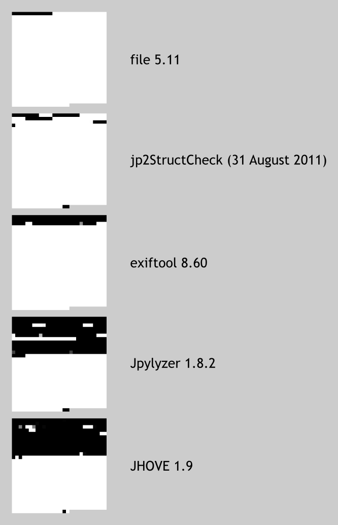
First, I looked at identification and characterisation tools, as shown below in order of increasing sensitivity:
For the file tool, which only performs identification, we can clearly see that it is only sensitive to the JPEG 2000 ‘magic number’ at the start of the file, and the remainder of the file is ignored completely. Note that DROID uses the same signature information, so can be expected to give the same result. However, we were not able to test this as at the time of the experiment, DROID did not lend itself well to being run repeatedly from the command line at high speed.
The other tools clearly perform deeper analyses. The next most sensitive one, jp2StructCheck, was the predecessor of Jpylyzer, and although clearly more sensitive than file, the sensitivity map is consistent with a basic structural analysis. The exiftool metadata extractor is much more sensitive to the file header, but unlike jp2StructCheck, does not inspect any other parts of the file at all.
Both Jyplyzer and JHOVE are sensitive to far more changes, and the advances made by Jpylyzer over jp2StructCheck are particularly striking. Interestingly, full JHOVE characterisation is sensitive to significantly more of the file than Jpylyzer, but appears to ignore parts of the file that Jpylyzer covers. None of these tools appear to be sensitive to much of the latter half of the file, confirming that this area corresponds to the actual compressed image data.
Validation
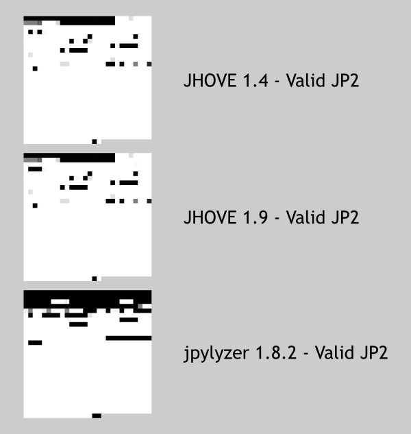
Here, we focussed only on the validation tools, and instead of using the whole characterisation output as ‘ground truth’, we just extract the ‘is Valid’ result and compare that. Therefore, these maps show which parts of the JP2 appear to be validated, not just extracted. For example, if there is a comment in the file, the characterisation process may notice that modifying it changes the text, but probably will not be able to say whether the comment text is valid or not.
We can see minor differences between JHOVE versions, indicating how this approach could be used to complement tool development and regression testing. More interestingly, it is clear that Jpylyzer is much more discerning than JHOVE in this regard. Many of input files that JHOVE would accept as valid are determined to be invalid by Jpylyzer, suggesting that it performs a more rigorous validation.
Rendering
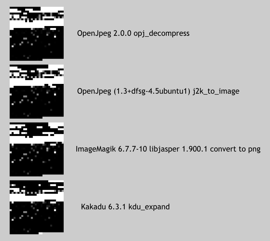
As mentioned above, it appears that none of the tools considered so far are able analyse or validate the actual compressed image data. We have seen the analysis of the file structure and the metadata, but to learn more, there is no alternative but to use an actual JP2 decompresser to convert the image to a different format, and check if the resulting image (if there is any) is modified when we flip the bits.
This shows that OpenJpeg, ImageMagick (JasPer), and Kakadu are all highly sensitive to the image data, but ignore changes to significant fractions of the header data that the characterisation tools did cover. This suggest that the best validation strategy may be to combine Jpylyzer with a JP2 decompresser, in order to maximise coverage of the image data and metadata. Similarly, deeper inspection of the characterisation tool results (such as outlined in the conclusions below) could be use to determine precisely what data is being discarded during the decompression.
Of these tools, Kakadu appears to be the most sensitive renderer, although it is a close call, and the maps within the image data area are very similar. Note that the small amounts of ‘ignored’ data in the image payload may correspond to errors that were noticed but were silently corrected.
Conclusions
On it’s own, this approach provides an interesting way to understand bitstreams and compare tools, although it would benefit from additional development to make it easier to compare and combine the sensitivity maps. Furthermore, the understanding of the bitstream itself can be deepened by monitoring the output of the tool more closely. For example, when working with characterisation tools, we can see directly if the bit we just flipped modified a comment, a colour-space, or some other data or metadata the tool is capable of exposing. A relatively simple user interface could use this approach to create an engaging way to explore bitstream data formats interactively.
These techniques could also form the basis of a sophisticated preservation tool regression testing and comparison system, which has the distinct advantage of having to invest very little knowledge up-front about the format itself. We only need to define the output of interest for a given tool or set of tools, and can put a range of different bitstreams through them in order to learn more about both. In essence, we trust the software to inform us about the format, and this can be used to kick-start the more traditional approach of documenting formats and creating format test suites. Tools could also be compared using this approach, e.g. in terms of how comprehensively each sensitivity map covers the input bitstream.
As indicated above, one limitation of this approach is that redundant data cannot be distinguished from ignored data. For a dedicated digital preservation tool, this should not be a major limitation, as such tools should not silently fix errors. However, when using a broader range of tools, we can start to compensated for this by learning more about the format and comparing different tools. In the work outlined here, it seems likely that the majority of the ‘insensitive’ data really is simply ignored, but further research would be required to come up with ways of understanding how to verify whether that is truly the case.
The main limitation of this approach is the high volume of computation time required by such intensive processing. Even for this very small 773 byte test file, each bitwise analysis involves running each tool 6184 times. This took around an hour per tool, although of course this depends on the nature tool (for example, Java tools tend to be slower than C tools). Further research could determine whether full byte-flips are an acceptable alternative to flipping each byte individually, although even given this eight-fold speed increase, the approach is only likely to be feasible for smaller files. However, the success of the approach does not depend on the size of the files, but rather on the degree to which the input files cover the features available in a given format. Further research, perhaps similar to this, could look at ways of analysing and mapping out how the software reacts to the input data.
There were a number of technical complications involved during the implementation of this approach which have not been documented here. If you are interested in those details, the source code and example data used in this experiment are available on GitHub.
On Tools


